Automatic Mixed Precision Training (AMP)¶

In general, the default datatype (dtype) of training deep learning model is float32, and each data occupies 32 bits of storage space. In order to save the consumption of memory, the industry has proposed 16 bit data types (such as float16 and bfloat16 supported by GPU). Each data only needs 16 bits storage space, saving half the storage space compared with float32. Some chips can obtain faster computing speed on 16 bit data. For example, according to the data of NVIDIA, On a V100 GPU, matrix multiply and convolution operations can be speeded up to 8x in float16 over their float32 equivalents.

Considering that some operators (OPS) require high data accuracy (such as softmax and cross_entropy), this kind of operator still needs to be calculated with float32. Some operators (such as conv2d and matmul) are not sensitive to data accuracy, float16 / bfloat16 can be used to improve the calculation speed and reduce the storage space, Paddle provides Automatic Mixed Precision (AMP), during model training, the appropriate data calculation accuracy (float32 or float16 / bfloat16) is automatically selected for the operator, which can accelerate the training without losing the training accuracy. Please refer to the papers jointly released by Baidu and NVIDIA in 2018: MIXED PRECISION TRAINING. This tutorial will introduce how to use automatic mixed precision training with PaddlePaddle.

I. overview¶

1.1. Floating datatype¶

Both float16 and bfloat16（brain floating point）are half precision floating-point data types that are stored in a computer using 2 bytes (16 bits). Compared with the single precision floating point number (float32) and double precision floating point number (float64) commonly used in calculation, float16 and bfloat16 are more suitable for use in scenarios with low precision requirements.

Compare the floating-point formats of float32 and float16 / bfloat16, as shown in Figure 1:

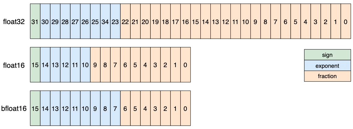
missing — Figure 1. Floating-point formats of float32 and float16 / bfloat16

The above data types have the following numerical characteristics:

The exponent bit of float32 is 8 bits and the fraction bit is 23 bits. The dynamic range of data that can be represented is [2^-126, 2^127], which is the default data type used in the deep learning model.
The exponent bit of float16 is 5 bits and the fraction bit is 10 bits. Compared with float32, the dynamic range of representable data is lower. The minimum representable positive number is 2^-14, and the maximum representable data is 65504, which is prone to numerical overflow.
The exponent bit of bfloat16 is 8 bits and the fraction is 7 bits. It is characterized by sacrificing accuracy to obtain a larger data range. The representable data range is consistent with float32. However, compared with float16, bfloat16 has lower data accuracy and is more prone to numerical underflow than float16.

1.2. AMP calculation process¶

1.2.1 auto_cast¶

Paddle adopts auto_cast strategy realizes the automatic conversion and use of calculation accuracy during model training. Generally, the model parameters are stored in the single precision floating-point format (float32). In the training process, the model parameters are converted from float32 to the half precision floating-point number (float16 or bfloat16) to participate in the forward calculation, and the half precision floating-point number represents the intermediate state. Then the half precision floating-point number is used to calculate the parameter gradient, and finally the parameter gradient is converted to the single precision floating-point number format, Update model parameters. The calculation process is shown in Figure 2 below:

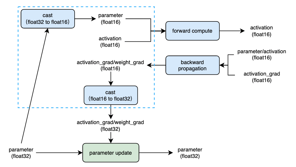
The logic in the blue dashed box in the figure2 is the parameter accuracy conversion (cast) logic under the amp policy. Generally, the overhead brought by cast operation is limited. When the computational performance benefit obtained by using float16 / bfloat16 in the process of forward compute and back propagation is greater than the overhead brought by cast, enabling amp training will get better training performance.

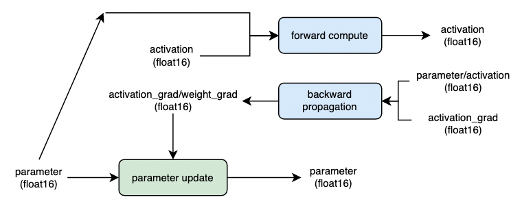
When the model parameters are stored in half precision floating-point format (float16 / bfloat16) before training, the cast operation in Figure 2 will be omitted in the training process, which can further improve the model training performance. However, it should be noted that the model parameters are stored in low precision data types, which may affect the final training accuracy of the model. The calculation process is shown in Figure 3 below:

1.2.2 grad_scaler¶

As mentioned in 1.1, the representation range of half precision floating-point numbers is much smaller than that of single precision floating-point numbers. In deep learning, the values of parameters, intermediate states and gradients are usually very small. Therefore, when half precision floating-point numbers are used to participate in the calculation, it is easy to cause underflow, that is, the underflow of values close to zero is zero. Paddle use the grad_scaler policy to avoid this problem: multiply the training loss by a loss_scaling value. According to the chain rule, in the back propagation process, the parameter gradient is also equivalent to multiplying loss_scaling. When the parameter is updated, the gradient value is divided by loss_scaling.

However, in the process of model training, select the appropriate loss_scaling value is a challenge, so Paddle provides dynamic loss_scaling: loss_scaling:

Before the training, for loss_scaling set a large initial value init_loss_scaling, default is 2^15, and set 4 parameters for dynamic adjustment loss_scaling: incr_ratio=2.0, decr_ratio=0.5, incr_every_n_steps=1000, decr_every_n_nan_or_inf=2;
After starting the training, after each calculation of the gradient, check all the gradients, judge whether there is nan/inf, and record the number of consecutive occurrences of nan/inf or the number of consecutive occurrences of nan/inf;
when nan/inf does not appear for incr_every_n_step consecutive iterations, multiply loss_scaling by incr_ratio;
when nan/inf occurs in decr_every_n_nan_or_inf consecutive iterations, multiply loss_scaling by decr_ratio;

1.3. AMP supported hardware¶

Paddle AMP supports following hardware, and the data type supported by different hardware is as follows:

硬件	支持的混合精度
Nvidia GPU	float16	bfloat16
Intel CPU	bfloat16
华为 NPU	float16
昆仑芯 XPU	float16
寒武纪 MLU	float16

Take NVIDIA GPU as an example to introduce the hardware acceleration mechanism:

When the same hyperparameters are used, mixed precision training using FP16/BF16 and FP32 can achieve the same accuracy as that of pure single precision used, and can accelerate the training speed.

It mainly attributes to the features that NVIDIA Volta and NVIDIA Turing use FP16 to calculate:

FP16 can reduce memory bandwidth and storage requirements by half, which allows researchers to use more complex models and larger batch sizes under the same hardware conditions.
FP16 can make full use of Tensor Cores technology provided by NVIDIA Volta Turing and Ampere. On the same GPU hardware, the computing throughput of Tensor Cores’ FP16 is 8 times bigger than that of FP32.

Starting from NVIDIA Ampere, GPU supports bfloat16, and its computing performance is the same as that of float16.

The nvidia-smi command can help you view NVIDIA GPU architecture information. AMP only support NVIDIA GPU with Compute Capability 7.0 or higher. In addition, if the amp training mode is enabled, PaddlePaddle will automatically help detect whether the hardware environment meets the above hardware conditions. If not, the following warning messages will be provided: UserWarning: AMP only support NVIDIA GPU with Compute Capability 7.0 or higher, current GPU is: Tesla K40m, with Compute Capability: 3.5..

1.4. Description of applicable scenarios¶

AMP usually needs to obtain higher benefits in the scenario of high memory utilization. Specifically, there are operators such as matmul and conv with large computational load in the model. If the proportion of the above operators in the model is relatively small, the benefit of AMP is very limited, at the same time, in order to use AMP, it will also bring the overhead of precision conversion (cast).

II. Dynamic graph training with AMP¶

Using PaddlePaddle’s API can realize automatic mixed precision training (AMP), which can automatically choose FP16 or FP32 for different operators’ calculation.

According to the use degree of FP16 in the model, the AMP is divided into two levels:

level = ’O1‘: The black&white operator list strategy is used for AMP. The op in the black list will be calculated by FP32, and the op in the white list will be calculated by FP16. During the training process, Paddle will automatically change the input data type of the op in the white list from FP32 to FP16. The operator list calculated by FP16 and FP32 can be found in this document.For an op that is not in the black&white list, Paddle will infer based on all the input data types of the op. when all the inputs are FP16, the op will directly use FP16 for calculation, otherwise FP32 for calculation. Refer to figure 2 for calculation logic.
level = ’O2‘: This mode adopts a more radical strategy than O1. Except ops that the Paddle does not support calculated by FP16, all other ops use FP16. Paddle will cast the neural network parameters from FP32 to FP16. Compared with O1, the training speed will be significantly improved, but there may be accuracy problems. Therefore, Paddle provides a user-defined blacklist through which you can specify some ops with accuracy problems to perform FP32 operations. Refer to figure 3 for calculation logic.

The dynamic graph training mode is recommended for Paddle. The following takes the dynamic graph single card (GPU) training code as an example to learn how to use Paddle basic API and the high-level API to realize AMP training.

2.1. Use basic API¶

Paddle Dynamic Graph provides a series of convenient APIs for AMP: paddle.amp.auto_cast and paddle.amp.GradScaler API。 Of which:

paddle.amp.auto_cast: used to create a context environment of AMP to support the AMP strategy of ops executed in Dynamic Graph.
paddle.amp.GradScaler: used to control the scaling ratio of loss and help avoid floating-point overflow (Note: optional, if FP16 data type is used to ensure that parameters will not overflow, it is not necessary to call this interface)

In AMP-O2 level, in addition to using the above two APIs, the paddle.amp.decorate is also used to convert the network parameters from float32 to float16, reducing cast operation in auto_cast logic.

2.1.1. FP32 training mode of Dynamic Graph¶

For comparison, this example first performs a common float32 training to compare the acceleration effect of AMP training.

1) Build a simple neural network by Paddle

In order to fully reflect the speed improvement brought by AMP, build a network composed of nine layers of linear. Each layer of linear network is composed of matmul and add operator. The matmul is an operator that can be accelerated.

            import time
import paddle
import paddle.nn as nn
import numpy

paddle.seed(100)
numpy.random.seed(100)
place = paddle.CUDAPlace(0)
# build a network composed of nine layers of linear
class SimpleNet(paddle.nn.Layer):
    def __init__(self, input_size, output_size):
        super().__init__()
        # nine layers of linear, each layer is composed of matmul and add operator
        self.linears = paddle.nn.LayerList(
            [paddle.nn.Linear(input_size, output_size) for i in range(9)])

    def forward(self, x):
        for i, l in enumerate(self.linears):
            x = self.linears[i](x)
        return x

           

2) Set relevant training parameters and training data

in order to effectively see the improvement of training speed by AMP, set the value of input_size and output_size to a larger value. In order to use the tensor core provided by the GPU, it is also necessary to set batch_size a multiple of 8.

            epochs = 2
input_size = 8192   # Set it to a larger value to compare the acceleration effect of AMP training more obviously
output_size = 8192  # Set it to a larger value to compare the acceleration effect of AMP training more obviously
batch_size = 2048   # batch_size is 8, the acceleration effect is better
nums_batch = 10

# Dataloader
from paddle.io import Dataset
class RandomDataset(Dataset):
    def __init__(self, num_samples):
        self.num_samples = num_samples

    def __getitem__(self, idx):
        data = numpy.random.random([input_size]).astype('float32')
        label = numpy.random.random([output_size]).astype('float32')
        return data, label

    def __len__(self):
        return self.num_samples

dataset = RandomDataset(nums_batch * batch_size)
loader = paddle.io.DataLoader(dataset, batch_size=batch_size, shuffle=False, drop_last=True, num_workers=0)

           

3) Using Dynamic Graph FP32 training

            mse = paddle.nn.MSELoss() # Define loss calculation function
model = SimpleNet(input_size, output_size) # Define SimpleNet model
optimizer = paddle.optimizer.SGD(learning_rate=0.0001, parameters=model.parameters()) # Define SGD optimizer

train_time = 0 # Record total training duration
for epoch in range(epochs):
    for i, (data, label) in enumerate(loader):
        start_time = time.time() # Record start time
        label._to(place) # Copy label to GPU
        # forward compute
        output = model(data)
        # loss compute
        loss = mse(output, label)
        # backward
        loss.backward()
        # update parameters
        optimizer.step()
        optimizer.clear_grad(set_to_zero=False)
        # record training loss and training time
        train_loss = loss.numpy()
        train_time += time.time() - start_time

print("loss:", train_loss)
print("Time consuming using FP32 mode:{:.3f} sec".format(train_time/(epochs*nums_batch)))
# loss: [0.6486028]
# Time consuming using FP32 mode:0.529 sec

           

Note: if the sample code shows an error related to out of memory on your machine, please try setting input_size、output_size、batch_size decrease.

2.1.2. AMP-O1 training mode of Dynamic Graph¶

In Paddle, two logics need to be added on the basis of FP32 code when AMP-O1 is used for training:

logic 1: use paddle.amp.auto_cast to create a context environment of AMP. In AMP context, Paddle will automatically determine the input data type (float32 or float16/bfloat16) of each OP according to the black&white list preset by Paddle. You can also add a custom_black_list OP list in this API.
logic 2: optional, use paddle.amp.Gradscaler to scale the loss to avoid floating-point underflow. Paddle turns on dynamic loss scaling by default, see 1.2.2 grad_scaler for details.

            mse = paddle.nn.MSELoss() # Define loss calculation function
model = SimpleNet(input_size, output_size) # Define SimpleNet model
optimizer = paddle.optimizer.SGD(learning_rate=0.0001, parameters=model.parameters()) # Define SGD optimizer

# logic 2: optional, use ``paddle.amp.Gradscaler`` to scale the ``loss`` to avoid floating-point underflow
scaler = paddle.amp.GradScaler(init_loss_scaling=1024)

train_time = 0 # Record total training duration
for epoch in range(epochs):
    for i, (data, label) in enumerate(loader):
        start_time = time.time() # Record start time
        label._to(place) # Copy label to GPU
        # logic 1: create a context environment of AMP, add elementwise_add op to custom_white_list so that all ops in forward will use float16
        with paddle.amp.auto_cast(custom_white_list={'elementwise_add'}, level='O1'):
            # forward compute
            output = model(data)
            # loss compute
            loss = mse(output, label)
        # logic 2: use GradScaler to scale the loss
        scaled = scaler.scale(loss) # loss scale, multiply by the coefficient loss_scaling
        scaled.backward() # backward
        scaler.step(optimizer)  # Update parameters (divide the parameter gradient by the coefficient loss_scaling and then update the parameters)
        scaler.update() # Based on dynamic loss_scaling policy update loss_scaling coefficient
        optimizer.clear_grad(set_to_zero=False)
        # record training loss and training time
        train_loss = loss.numpy()
        train_time += time.time() - start_time

print("loss:", train_loss)
print("Time consuming using AMP-O1 mode:{:.3f} sec".format(train_time/(epochs*nums_batch)))
# loss: [0.6486219]
# Time consuming using AMP-O1 mode:0.118 sec

           

2.1.3. AMP-O2 training mode of Dynamic Graph¶

AMP-O2 need to add three logics on the basis of FP32 code:

logic 1: use paddle.amp.decorate cast network parameters from FP32 to FP16.
logic 2: use paddle.amp.auto_cast to create a context environment of AMP，Paddle will use FP16 to calculate all ops except the customized blacklist.
logic 3: optional, use paddle.amp.Gradscaler to scale the loss to avoid floating-point underflow.

            mse = paddle.nn.MSELoss() # Define loss calculation function
model = SimpleNet(input_size, output_size) # Define SimpleNet model
optimizer = paddle.optimizer.SGD(learning_rate=0.0001, parameters=model.parameters()) # Define SGD optimizer

# logic 1: cast network parameters from FP32 to FP16.
model = paddle.amp.decorate(models=model, level='O2')

# logic 3: optional,  use GradScaler to scale the ``loss`` to avoid floating-point underflow
scaler = paddle.amp.GradScaler(init_loss_scaling=1024)

train_time = 0 # Record total training duration
for epoch in range(epochs):
    for i, (data, label) in enumerate(loader):
        start_time = time.time()
        label._to(place) # Copy label to GPU
        # logic 2: create a context environment of AMP, all ops in forward will use float16
        with paddle.amp.auto_cast(level='O2'):
            # forward compute
            output = model(data)
            # loss compute
            loss = mse(output, label)
         # logic 3: use GradScaler to scale the loss
        scaled = scaler.scale(loss) # loss scale, multiply by the coefficient loss_scaling
        scaled.backward() # backward
        scaler.step(optimizer) # Update parameters (divide the parameter gradient by the coefficient loss_scaling and then update the parameters)
        scaler.update() # Based on dynamic loss_scaling policy update loss_scaling coefficient
        optimizer.clear_grad(set_to_zero=False)
        # record training loss and training time
        train_loss = loss.numpy()
        train_time += time.time() - start_time

print("loss=", train_loss)
print("Time consuming using AMP-O2 mode:{:.3f} sec".format(train_time/(epochs*nums_batch)))
# loss= [0.6743]
# Time consuming using AMP-O2 mode:0.102 sec

           

2.1.4. Compare training speed in different modes¶

The comparison of the accuracy and speed of float32 and AMP training is shown in the following table:

-	float32	AMP-O1	AMP-O2
Time consuming	0.529s	0.118s	0.102s
loss	0.6486028	0.6486219	0.6743

It can be seen from the statistical results in the above table that the training speed in O1 mode is increased by about 4.5 times, and that in O2 mode is increased by about 5.2 times.

The above example build an idealized experimental model. The acceleration is obvious because the proportion of matmul operator is relatively high. The acceleration effect of the actual model is related to the characteristics of the model. In theory, the acceleration effect of models with high proportion of matmul and conv is more obvious. In addition, due to the machine environment, the training time statistics of the above example codes may be different. The impact mainly includes: GPU utilization, CPU utilization, etc. the test machine configuration is as follows:

Device	MEM Clocks	SM Clocks	Running with CPU Clocks
Tesla V100 SXM2 16GB	877 MHz	1530 MHz	1000 - 2400 MHz

2.2. Use high level API¶

The new high-level API launched by Paddle 2.0 is a further package and upgrade of the basic API. It provides a more concise and easy-to-use API, improves the ease of learning and use of Paddle, and enhances the functions of Paddle. Examples of AMP usage in high-level APIs are as follows, AMP configurations are mainly imported through the amp_configs parameter of paddle.Model.prepare.

           import paddle
import paddle.nn as nn
import paddle.vision.transforms as T

def run_example_code():
    device = paddle.set_device('gpu')
    # Using high level API to define neural network
    net = nn.Sequential(nn.Flatten(1), nn.Linear(784, 200), nn.Tanh(), nn.Linear(200, 10))
    model = paddle.Model(net)
    # Define optimizer
    optim = paddle.optimizer.SGD(learning_rate=1e-3, parameters=model.parameters())
    # Initialize neural network
    amp_configs = {
        "level": "O1",                    # Level corresponds to amp mode: O1, O2
        "custom_white_list": {'conv2d'},  # Customize the white list and support custom_black_list
        "use_dynamic_loss_scaling": True  # Dynamic loss_scaling
    }
    model.prepare(optim,
        paddle.nn.CrossEntropyLoss(),
        paddle.metric.Accuracy(),
        amp_configs=amp_configs)
    # prepare data
    transform = T.Compose([T.Transpose(), T.Normalize([127.5], [127.5])])
    data = paddle.vision.datasets.MNIST(mode='train', transform=transform)
    # use AMP training
    model.fit(data, epochs=2, batch_size=32, verbose=1)

if paddle.is_compiled_with_cuda():
    run_example_code()

          

III. Other usage scenarios¶

The previous article introduced the method of single card (GPU) training in dynamic graph mode, which is similar to it, distributed training documents and dynamic graph to static graph can start AMP in the same way. Next, it mainly introduces the methods of starting AMP training in static graph modes and the advanced usage of AMP training, such as gradient accumulation.

3.1 Gradient Accumulation in dynamic graph mode¶

Gradient accumulation means running a configured number of steps without updating the model variables. Until certain steps, use the accumulated gradients to update the variables. Limited by the size of the gpu memory, you may not be able to open a larger batch_size, you can increase batch_size by using gradient accumulation.

In automatic mixed precision training, gradient accumulation is also supported, and the usage is as follows:

           mse = paddle.nn.MSELoss() # Define loss calculation function
model = SimpleNet(input_size, output_size)  # Define SimpleNet model
optimizer = paddle.optimizer.SGD(learning_rate=0.0001, parameters=model.parameters())  # Define SGD optimizer

accumulate_batchs_num = 10 # the batch numbers of gradients accumulation

# define GradScaler
scaler = paddle.amp.GradScaler(init_loss_scaling=1024)

train_time = 0
for epoch in range(epochs):
    for i, (data, label) in enumerate(loader):
        start_time = time.time() # get start time
        label._to(place) # Copy label to GPU
         # create AMP context environment
        with paddle.amp.auto_cast(level='O1'):
            output = model(data)
            loss = mse(output, label)
        # use GradScaler complete the loss scaling
        scaled = scaler.scale(loss)
        scaled.backward()

        #  when the accumulated batch is accumulate_batchs_num, update the model parameters
        if (i + 1) % accumulate_batchs_num == 0:
            # update parameters
            scaler.step(optimizer)
            scaler.update()
            optimizer.clear_grad(set_to_zero=False)
        # record training loss and training time
        train_loss = loss.numpy()
        train_time += time.time() - start_time

print("loss:", train_loss)
print("Time consuming using AMP-O1 mode:{:.3f} sec".format(train_time/(epochs*nums_batch)))
# loss: [0.6602017]
# Time consuming using AMP-O1 mode:0.113 sec

          

In the above example, after accumulate_batchs_num batch training steps, with one parameter update.

3.2. AMP in Static Graph¶

Paddle starts AMP training in Static Graph, the compute logic is similar to the dynamic graph, except that the called interfaces are different. Paddle Static Graph provides a series of convenient APIs for AMP: paddle.static.amp.decorate, paddle.static.amp.fp16_guard.

paddle.static.amp.decorate: Decorate the optimizer, add amp logic, and set the parameters of grad_scaler through this API.
paddle.static.amp.fp16_guard: In AMP_O2 mode, the scope of float16 is controlled only in context manager fp16_guard.

3.2.1. FP32 training mode of Static Graph¶

Adopt the same network structure as Dynamic Graph training in section 2.1.1.

            paddle.enable_static() # Enable static graph mode
place = paddle.CUDAPlace(0)
# Define the static program
main_program = paddle.static.default_main_program()
startup_program = paddle.static.default_startup_program()
# Define a neural network consisting of 9 layers of linear
model = SimpleNet(input_size, output_size)
# Define loss function
mse_loss = paddle.nn.MSELoss()

           

Static Graph training code is as follows:

            # Define training data and labels
data = paddle.static.data(name='data', shape=[batch_size, input_size], dtype='float32')
label = paddle.static.data(name='label', shape=[batch_size, input_size], dtype='float32')
# forward
predict = model(data)
# compute loss
loss = mse_loss(predict, label)
# Define optimizer
optimizer = paddle.optimizer.SGD(learning_rate=0.0001, parameters=model.parameters())
optimizer.minimize(loss)
# Define static diagram executor
exe = paddle.static.Executor(place)
exe.run(startup_program)

train_time = 0 # Record total training duration
for epoch in range(epochs):
    for i, (train_data, train_label) in enumerate(loader()):
        start_time = time.time() # Record start time
        # Executive Training
        train_loss = exe.run(main_program, feed={data.name: train_data, label.name: train_label }, fetch_list=[loss.name], use_program_cache=True)
        # Record training duration
        train_time += time.time() - start_time

print("loss:", train_loss)
print("Time consuming using FP32 mode:{:.3f} sec".format(train_time/(epochs*nums_batch)))
loss: [array([0.6486028], dtype=float32)]
Time consuming using FP32 mode:0.531 sec

           

3.2.2. AMP-O1 training mode of Static Graph¶

The Static Graph uses paddle.static.amp.decorate to decorate the optimizer and use paddle.static.amp.CustomOpLists to define the black&white list to start the AMP training. The example code is as follows:

            # Define training data and labels
data = paddle.static.data(name='data', shape=[batch_size, input_size], dtype='float32')
label = paddle.static.data(name='label', shape=[batch_size, input_size], dtype='float32')
# forward
predict = model(data)
# compute loss
loss = mse_loss(predict, label)
# Define optimizer
optimizer = paddle.optimizer.SGD(learning_rate=0.0001, parameters=model.parameters())

# 1) use `CustomOpLists` to define Black and white lists
amp_list = paddle.static.amp.CustomOpLists(custom_white_list=['elementwise_add'])

# 2）decorate the optimizer for amp:
optimizer = paddle.static.amp.decorate(
    optimizer=optimizer,
    amp_lists=amp_list,
    init_loss_scaling=128.0,
    use_dynamic_loss_scaling=True)

optimizer.minimize(loss)
# Define static diagram executor
exe = paddle.static.Executor(place)
exe.run(startup_program)

train_time = 0 # Record total training duration
for epoch in range(epochs):
    for i, (train_data, train_label) in enumerate(loader()):
        start_time = time.time() # Record start time
        # Executive Training
        train_loss = exe.run(main_program, feed={data.name: train_data, label.name: train_label }, fetch_list=[loss.name], use_program_cache=True)
        # Record training duration
        train_time += time.time() - start_time

print("loss:", train_loss)
print("Time consuming using AMP-O1 mode:{:.3f} sec".format(train_time/(epochs*nums_batch)))
loss: [array([0.6486222], dtype=float32)]
Time consuming using AMP-O1 mode:0.117 sec

           

paddle.static.amp.CustomOpLists is used to customize the black-and-white list. The black list OP implements float32 kernel and the white list OP implements float16 kernel. Elementwise_add op is added in custom_white_list, so that Linear will compute in float16.

3.2.3. AMP-O2 training mode of Static Graph¶

There are two ways to start AMP-O2 in Static Graph:

use paddle.static.amp.fp16_guard to control the scope of FP16 application. All ops in this context will perform FP16 calculation, and other OPS will perform FP32 calculation;
not usepaddle.static.amp.fp16_guard to control the scope of FP16 application. All the ops of the network perform FP16 calculation (excluding the ops in the user-defined blacklist and those that do not support FP16 calculation)

Set paddle.static.amp.decorate parameter use_pure_fp16 is True, and the parameter use_fp16_guard is False

            data = paddle.static.data(name='data', shape=[batch_size, input_size], dtype='float32')
label = paddle.static.data(name='label', shape=[batch_size, input_size], dtype='float32')

predict = model(data)
loss = mse_loss(predict, label)

optimizer = paddle.optimizer.SGD(learning_rate=0.0001, parameters=model.parameters())

# 1）decorate the optimizer for amp:
optimizer = paddle.static.amp.decorate(
    optimizer=optimizer,
    init_loss_scaling=128.0,
    use_dynamic_loss_scaling=True,
    use_pure_fp16=True,
    use_fp16_guard=False)

optimizer.minimize(loss)

exe = paddle.static.Executor(place)
exe.run(startup_program)

# 2) use `amp_init` convert FP32 parameters of the network to FP16
optimizer.amp_init(place, scope=paddle.static.global_scope())

train_time = 0 # Record total training duration
for epoch in range(epochs):
    for i, (train_data, train_label) in enumerate(loader()):
        start_time = time.time() # Record start time
        # Executive Training
        train_loss = exe.run(main_program, feed={data.name: train_data, label.name: train_label }, fetch_list=[loss.name], use_program_cache=True)
        # Record training duration
        train_time += time.time() - start_time

print("loss:", train_loss)
print("Time consuming using AMP-O2 mode:{:.3f} sec".format(train_time/(epochs*nums_batch)))
loss: [array([0.6743], dtype=float16)]
Time consuming using AMP-O2 mode:0.098 sec

           

Note: in AMP-O2 mode, the network parameters will be changed from FP32 to FP16. The input data needs to be FP16 data type. Therefore, the data type initialized in the class randomdataset needs to be set to float16.

Set paddle.static.amp.decorate parameter use_pure_fp16 is True, and the parameter use_fp16_guard is true, and use paddle.static.amp.fp16_guard control the calculation range of FP16.

Add code to model definition fp16_guard control part of network execution under FP16:

            class SimpleNet(paddle.nn.Layer):
    def __init__(self, input_size, output_size):
        super().__init__()
        self.linears = paddle.nn.LayerList(
            [paddle.nn.Linear(input_size, output_size) for i in range(9)])

    def forward(self, x):
        for i, l in enumerate(self.linears):
            if i > 0:
                # Through fp16_guard controls the calculation range using float16
                with paddle.static.amp.fp16_guard():
                    x = self.linears[i](x)
            else:
                x = self.linears[i](x)
        return x

           

The training codes in this mode are as follows:

            data = paddle.static.data(name='data', shape=[batch_size, input_size], dtype='float32')
label = paddle.static.data(name='label', shape=[batch_size, input_size], dtype='float32')

predict = model(data)
loss = mse_loss(predict, label)

optimizer = paddle.optimizer.SGD(learning_rate=0.0001, parameters=model.parameters())

# 1）decorate the optimizer for amp:
optimizer = paddle.static.amp.decorate(
    optimizer=optimizer,
    init_loss_scaling=128.0,
    use_dynamic_loss_scaling=True,
    use_pure_fp16=True,
    use_fp16_guard=True)

optimizer.minimize(loss)

exe = paddle.static.Executor(place)
exe.run(startup_program)

# 2) use `amp_init` convert FP32 parameters of the network to FP16
optimizer.amp_init(place, scope=paddle.static.global_scope())

train_time = 0 # Record total training duration
for epoch in range(epochs):
    for i, (train_data, train_label) in enumerate(loader()):
        start_time = time.time() # Record start time
        # Executive Training
        train_loss = exe.run(main_program, feed={data.name: train_data, label.name: train_label }, fetch_list=[loss.name], use_program_cache=True)
        # Record training duration
        train_time += time.time() - start_time

print("loss:", train_loss)
print("Time consuming using AMP-O2 mode:{:.3f} sec".format(train_time/(epochs*nums_batch)))
loss: [array([0.6691731], dtype=float32)]
Time consuming using AMP-O2 mode:0.140 sec

           

3.2.4. Compare training speed in different modes¶

The comparison of accuracy and speed of Static Graph FP32 and AMP training is shown in the following table:

-	FP32	AMP-O1	AMP-O2
Time consuming	0.531s	0.117s	0.098s
loss	0.6486028	0.6486222	0.6743

It can be seen from the statistical results in the above table that the training speed in O1 mode is increased by about 4.5 times, and that in O2 mode is increased by about 5.4 times.

IV. Other precautions¶

The fundamental reason why the Paddle AMP improves the training performance of the model is that: the Tensor Core is used to accelerate the matmul and conv under FP16. In order to obtain the best acceleration effect, the Tensor Core has certain use constraints on matrix multiplication and convolution operations. The constraints are as follows:

General matrix multiplication (GEMM) is defined as: C = A * B + C, of which:
- The dimension of matrix A is: M x K
- The dimension of matrix B is: K x N
- The dimension of matrix C is: M x N
Suggestion for matrix multiplication is: According to the Tensor Core usage recommendations, when the matrix dimensions of M, N, and K are multiples of 8 (the A100 architecture GPU is 16) (FP16 data), the performance is optimal.
Convolution is defined as: NKPQ = NCHW * KCRS, of which:
- N: batch size
- K: Number of output channels
- P: Number of output height
- Q: Number of output width
- C: Number of input channels
- H: Number of input height
- W: Number of input width
- R: Number of filter height
- S: Number of filter width
Suggestions for convolution are:
- The number of input and output channels（C/K) to be divisible by 8 (for FP16)（Cudnn7.6.3 and above will be automatically filled if it is not a multiple of 8）
- For the first layer of the network, setting the number of channels to 4 can obtain the best operation performance (NVIDIA provides a special implementation for the convolution of the first layer of the network, and the performance is better when using 4 channels)
- Set the tensor layout in memory to NHWC format (if NCHW format is input, the Tesor Core will be automatically converted to NHWC. When the input and output values are large, the cost of this conversion is often greater)

V. AMP common problems and Solutions¶

Common problems and treatment methods of Paddle AMP:

No acceleration effect or speed decrease after AMP Training:

Possible cause 1: The used GPU does not support AMP acceleration. You can view the following warning information in the training log: UserWarning: AMP only support NVIDIA GPU with Compute Capability 7.0 or higher, current GPU is: Tesla K40m, with Compute Capability: 3.5.;

Possible cause 2: The model is light computing and heavy scheduling, and the operations such as matmul and conv with large computing load account for a relatively low proportion. The utilization of GPU memory (Memory Usage and GPU_Util parameters) can be seen through nvidia-smi real-time production.

For the above reasons, it is recommended to turn off the hybrid accuracy training.
Runtimeerror thrown when AMP-O2 is used together with distributed training: For distributed AMP training, you should first use paddle.amp.decorate() to decotate origin model, and then call paddle.DataParallel get distributed model.

Cause: distributed training of AMP-O2 requires paddle.amp.decorate needs to be declared before the paddle.Dataparallel initializing the distributed training network.

The correct usage is as follows:

          import paddle
model = SimpleNet(input_size, output_size)  # Define loss calculation function
model = paddle.amp.decorate(models=model, level='O2') # paddle.amp.decorate needs to be declared before the paddle.Dataparallel
dp_model = paddle.DataParallel(model)

         